Equilibrating simulations

In this tutorial we will explain what equilibration of a simulation is and how MDMC can ensure enough equilibration has been done before running the simulation.

What is equilibration?

Equilibration of a simulation involves running the simulation for a period of time to make it ready for a ‘production run’ (i.e. one in which we record trajectories).

When the simulation is first set up, it has usually been configured in a certain way such as having atoms spaced in a grid at certain densities. We don’t want this to affect our trajectories, and we also want properties like kinetic and potential energies to be distributed around the simulation so that it better reflects the ‘real-life’ behaviour of molecules.

First, let us create and minimize an MDMC Simulation. Minimization, like equilibration, is a short run of the MD simulation which resolves issues like atoms overlapping (which would affect energy readings for the simulation).

import numpy as np

from MDMC.MD import Universe, Simulation, Atom, NonBonded, NonBondedForce
from openmm import unit

# create the topology
universe = Universe(dimensions=38.4441)
Ar = Atom('Ar', charge=0., mass=36.0)
n_ar_atoms = int(0.0176 * np.prod(universe.dimensions))
print(n_ar_atoms)
universe.fill(Ar, num_struc_units=(n_ar_atoms))

# define intermolecular forces
Ar_dispersion = NonBondedForce(universe,
                          Ar.atom_type,
                          cutoff=8.,
                          ewald=1e-6,
                          function=NonBonded(charge=0.0, epsilon=1.0243, sigma=3.36))

# MD Engine setup
simulation = Simulation(universe,
                        engine="openmm",
                        time_step=10.18893,
                        temperature=120.,
                        traj_step=15,
                        openmm_ensembles=[
                            # equilibration stage - equilibrate the cell volume and temperature
                            # with high friction and frequent Monte Carlo pressure changes
                            {
                                "integrator": "LangevinMiddle",
                                "frictionCoeff": 1.0 / unit.picoseconds,
                                "barostat": {
                                    "barostat": "MonteCarlo",
                                    # https://journals.aps.org/pra/pdf/10.1103/PhysRevA.31.3391
                                    # table 2 measurement (a) 2.01 MPa
                                    "defaultPressure": 20.1 * unit.bar,
                                    "frequency": 25
                                },
                                # runs auto-equilibration using the KPSS test on certain properties
                                # this tuple can be replaced with an int if you prefer to run
                                # a specific number of steps instead.
                                # auto-equilibration parameters are as follows:
                                # (ensemble [NPT runs KPSS test on volume and temperature],
                                # max number of steps, steps per iteration, kpss window,
                                # kpss tolerance)
                                "n_steps": ("NPT", 100000, 100, 1000, 0.01)
                            },
                            # production stage - not used here
                            {
                                "integrator": "LangevinMiddle",
                                "frictionCoeff": 1.0 / unit.picoseconds,
                            }
                        ])

Universe created with:
Dimensions [38.44 38.44 38.44]
1000
Simulation created with openmm engine and settings:
temperature: 120.0 K
openmm_ensembles: [{'integrator': 'LangevinMiddle', 'frictionCoeff': 1.0 /ps, 'barostat': {'barostat': 'MonteCarlo', 'defaultPressure': 20.1 bar, 'frequency': 25}, 'n_steps': ('NPT', 100000, 100, 1000, 0.01)}, {'integrator': 'LangevinMiddle', 'frictionCoeff': 1.0 /ps}]

We can then equilibrate the simulation. This is done by setting "n_steps": ("NPT", 100000, 100, 1000, 0.01) above and using with equilibration=True in simulation.run(n_steps=1, equilibration=True) note that the n_steps in simulation.run is ignored as the maximum steps is specified in the settings tuple.

We create a plot function so we can use it later.

import matplotlib.pyplot as plt
import numpy as np

def plot_vars(volumes, temperatures, energies, line=0):
    plt.figure()
    plt.subplot(311)
    plt.plot(np.arange(len(volumes))*10, volumes)
    plt.ylabel('Volumes')
    if line:
        plt.axvline(x=line, linestyle='--', color='lime')

    plt.subplot(312)
    plt.plot(np.arange(len(temperatures))*10, temperatures)
    plt.ylabel('Temperature (K)')
    if line:
        plt.axvline(x=line, linestyle='--', color='lime')

    plt.subplot(313)
    plt.plot(np.arange(len(energies))*10, energies, color="orange")
    plt.xlabel('time (steps)')
    plt.ylabel('Total energy (kJ/mol)')
    if line:
        plt.axvline(x=line, linestyle='--', color='lime')

    plt.show()

Avoiding under- or over- equilibrating

If we under-equilibrate, then it will affect our observed trajectory when we run the simulation. If we over-equilibrate, then we can waste time. How can we detect, on the fly, when our system is equilibrated?

MDMC features ‘auto-equilibration’, which analyses how variables change as equilibration progresses, and automatically halts the equilibration when it has determined these variables to be stationary. User-defined parameters can determine the sensitivity of this, as well as what is analysed.

To auto-equilibrate, create a simulation and then run simulation.engine.autoequilibrate. It returns the number of steps it used to equilibrate as well as data for the tracked variables.

simulation.engine.add_barostat(simulation.engine.openmm_ensembles[0]["barostat"])
total_steps, vals_dict = simulation.engine.autoequilibrate(*simulation.engine.openmm_ensembles[0]["n_steps"])

NPT ensemble auto-equilibration has detected stability after 9400 equilibration steps.

auto_vols = vals_dict['volumes']
auto_temperatures = vals_dict['temperatures']
auto_energies = vals_dict['total_energies']

plot_vars(auto_vols, auto_temperatures, auto_energies)

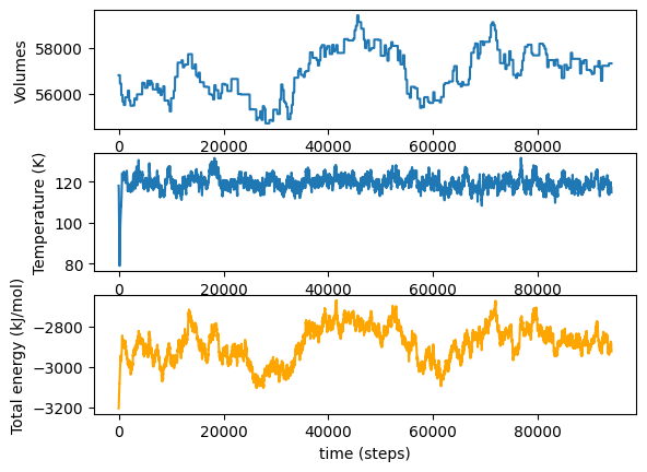
Try changing the values in "n_steps": ("NPT", 100000, 100, 1000, 0.01) or increasing you simulation size universe = Universe(dimensions=38.4441) and rerunning.