Usage with Euphonic and ResINS: TOSCA simulation

Mantid-Abins-like second-order almost-isotropic phonons for TOSCA

Gather phonon displacement data

Phonon frequencies and eigenvectors are loaded here from a CASTEP .phonon file and converted to sets of thermally-occupied 3x3 displacement tensors

from euphonic import QpointPhononModes, Quantity
import matplotlib.pyplot as plt
import numpy as np

from abinslib.almost_isotropic_incoherent import (
    calculate_almost_isotropic_incoherent_spectra,
    mantid_like_combination_spectra,
)
from abinslib.data import get_data
from abinslib.displacements import Displacements

# Get sample data; NaH phonon modes computed with CASTEP
castep_file = get_data("NaH.phonon")
modes = QpointPhononModes.from_castep(castep_file)

# Define simulation temperature using Pint units
temperature = Quantity(50, "kelvin")

# Create thermal displacement data from phonon eigenvectors
mode_displacements = Displacements.from_modes(modes, temperature=temperature)

# Compute average displacement over modes (mainly used for Debye-Waller factor)
atomic_displacements = mode_displacements.to_atomic_displacements()

Downloading file 'NaH.phonon' from 'https://github.com/pace-neutrons/Euphonic/raw/master/tests_and_analysis/test/data/castep_files/NaH/NaH.phonon' to '/home/runner/.cache/abinslib'.

Set up TOSCA kinematic constraints

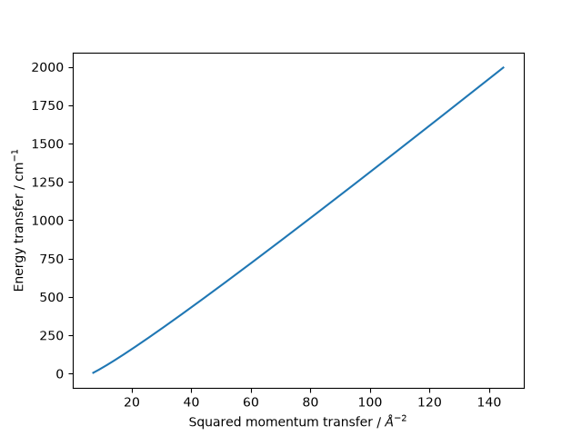
The indirect-geometry instrument TOSCA has detector banks at 45° and 135°; combined with the analyzer-determined final energy this constrains the accessible Q at each measured energy transfer.

For the fundamental spectrum we need a value of $Q^2$ for each input mode as these are used in the mode-by-mode Debye-Waller factor calculation

from abinslib.util import calculate_indirect_q2

tosca_backward_q2 = calculate_indirect_q2(
    modes.frequencies,
    angle=(135 * np.pi / 180),
    final_energy=Quantity(32.0, "cm^-1").to("hartree"),
)

For the multi-phonon spectrum the Q-dependent terms are applied as a correction after binning, so we supply the $Q^2$ values for the bins kinstead.

bins = Quantity(np.linspace(0, 2000, 201), "cm^-1")
bin_centres = (bins[1:] + bins[:-1]) * 0.5
binned_q2 = calculate_indirect_q2(
    bin_centres,
    angle=(135 * np.pi / 180),
    final_energy=Quantity(32.0, "cm^-1").to("hartree"),
)

fig, ax = plt.subplots()
ax.plot(binned_q2.to("angstrom^-2").magnitude, bin_centres.to("cm^-1").magnitude)
ax.set_xlabel(r"Squared momentum transfer / $\AA{}^{-2}$")
ax.set_ylabel(r"Energy transfer / cm$^{-1}$")

plt.show()

Calculate spectra

Calculate the fundamental and combination-mode intensities, binned to an output energy-transfer mesh.

fundamentals = calculate_almost_isotropic_incoherent_spectra(
    modes=modes,
    mode_displacements=mode_displacements,
    atomic_displacements=atomic_displacements,
    nominal_q2=tosca_backward_q2,
    bins=bins,
    apply_cross_section=True,
)

second_order = mantid_like_combination_spectra(
    modes,
    mode_displacements,
    atomic_displacements,
    binned_q2,
    bins,
    apply_cross_section=True,
)

spectra = fundamentals + second_order

Found reference data for H to match input symbol H with mass 1.00794.
Found reference data for Na-23 to match input symbol Na with mass 22.98977.
Found reference data for H to match input symbol H with mass 1.00794.
Found reference data for Na-23 to match input symbol Na with mass 22.98977.
Found reference data for H to match input symbol H with mass 1.00794.
Found reference data for Na-23 to match input symbol Na with mass 22.98977.

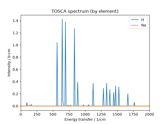
Plot spectra

Euphonic includes some convenience functions for plotting Spectrum objects. The SpectrumCollection1D class has a useful group_by(), select() and sum() methods which can be used to collect the desired plotting groups from a larger collection of components, using its .metadata.

from euphonic.plot import plot_1d_to_axis

fig, ax = plt.subplots()
for spectrum in spectra.group_by("atom_symbol"):
    plot_1d_to_axis(
        spectrum,
        ax=ax,
        label=spectrum.metadata["atom_symbol"],
    )

ax.legend()
ax.set_title("TOSCA spectrum (by element)")


def set_labels(ax, spectrum) -> None:
    ax.set_xlabel(f"Energy transfer / {spectrum.x_data.units:~^P}")
    ax.set_ylabel(f"Intensity / {spectrum.y_data.units:~^P}")


set_labels(ax, spectra)

plt.show()

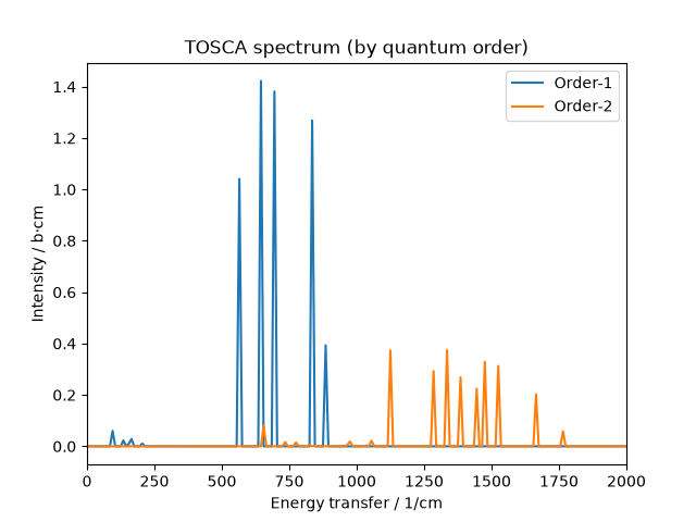
In practice the most useful divisions are by element or by quantum order

fig, ax = plt.subplots()
for spectrum in spectra.group_by("quantum_order"):
    plot_1d_to_axis(
        spectrum,
        ax=ax,
        label=f"Order-{spectrum.metadata['quantum_order']}",
    )

ax.legend()
ax.set_title("TOSCA spectrum (by quantum order)")
set_labels(ax, spectra)

plt.show()

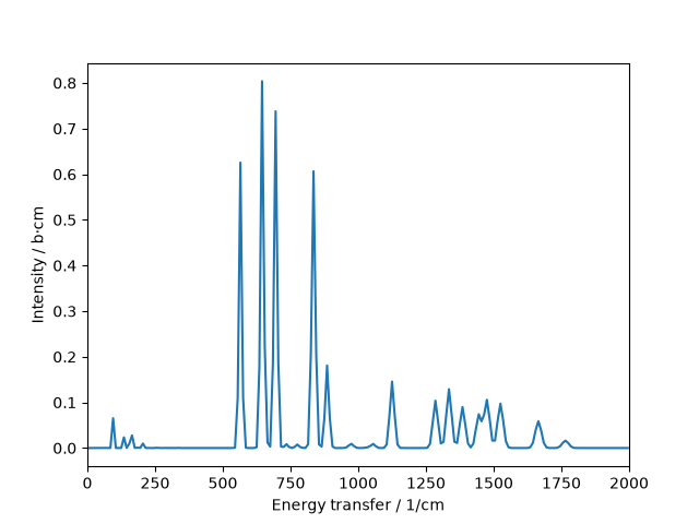
Sum contributions and apply resolution broadening

The resolution function of TOSCA is energy-dependent. An established approximation is implemented in the ResINS library; a variable-width Gaussian parametrised with a quadratic function.

from euphonic.plot import plot_1d
from resins import Instrument

tosca = Instrument.from_default("TOSCA")
res = tosca.get_resolution_function("AbINS_v1")

x = spectra.get_bin_centres().to("meV").magnitude
spectrum = spectra.sum()
y = spectrum.y_data.magnitude

y_broadened = res.broaden(
    # broaden() requires a Nx1 array of input points, so we broadcast a new
    # axis with None; in theory these could be 2D (|Q|,ω) or 4D (q,ω).
    points=x[:, None],
    data=y,
    # In this case the output mesh is the same as the input x-values
    mesh=x,
)
spectrum.y_data = Quantity(y_broadened, spectrum.y_data.units)

fig = plot_1d(spectrum)
set_labels(fig.axes[0], spectrum)
plt.show()